
If your firmware charges a battery from a solar panel, the interesting code only runs when the light changes. A cloud passes over, the current drops, the panel's voltage collapses, and your MPPT algorithm has to notice and back off. That is hard to test on a bench. You can't schedule weather, and you certainly can't reproduce the same cloud twice in CI.
The obvious substitute is a bench power supply set to the panel's rated voltage. It doesn't work, and it's worth being precise about why.
A panel is not a voltage source
A photovoltaic cell is a light-driven current source sitting in parallel with a diode. The light sets how much current is on offer (the short-circuit current, Isc). Draw less than that and the surplus flows through the diode, which holds the terminal voltage up near its open-circuit value, Voc. Draw close to all of it and the diode current falls away, and the voltage goes with it.
Plot that and you get the I-V curve: flat for most of its range, then a knee, then a cliff. A bench supply is flat everywhere and current-limits abruptly. It will never put your charger in the situation that actually exercises its control loop.
So we set out to make the BenchPod be a panel. Give it an I-V curve, and let it sag under load exactly where a real panel would.
The DAC can set a voltage, but it can't source current
The BenchPod's 16-bit DAC is an instrumentation output. It sets a precise voltage, but it is signal-level, so it can't supply the hundreds of milliamps a panel emulator needs to deliver. A panel is the current source in this story, and that part has to be built.
The external stage is three components:
- A TLV9152 op-amp, taking the DAC output as its setpoint
- An IRLZ44N logic-level MOSFET as the pass element, sourcing real current from a 9 V rail
- Four 0.01 ohm shunt resistors in series (40 mΩ nominal) with an INA282 current-sense amplifier at a fixed 50 V/V, feeding the reading back into the BenchPod's ADC
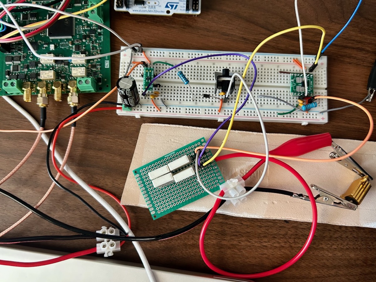
The detail that matters is where the op-amp takes its feedback: from the load side of the shunt. That puts the shunt's own voltage drop inside the regulation loop, so the DUT sees the panel voltage we asked for rather than that voltage minus whatever the sense resistor took.
One warning if you build this. The MOSFET is a linear pass element, so everything between the 9 V rail and the panel voltage burns inside it. At our full-sun operating point that is 4.8 V across the FET at 830 mA, so about 4 W, and the worst case sits right in the middle of the range. A bare TO-220 in still air would end up well over 200 °C above ambient. It needs a heatsink, which is why there is one in the photo.
Calibrating the current sense
The sense chain turns amps into millivolts, and the arithmetic is friendlier than it looks. 1 mA through R ohms drops exactly R millivolts, so after an amplifier gain of G the sensitivity is just R × G millivolts per milliamp. For a 45 mΩ shunt into the INA282's fixed 50 V/V, that comes to about 2.26 mV/mA.
Two things caught us out here, and both are worth repeating because they cost real time.
The shunt is not its marked value. Four 10 mΩ resistors in series should be 40 mΩ. Measured directly, the chain reads 45 mΩ. The extra 12% is perfboard interconnect and solder joints sitting inside the Kelvin sense taps. That's harmless as long as you calibrate the whole chain instead of trusting the part numbers, but it will quietly bias everything if you don't.
Don't infer the quantity you are trying to measure. Our first calibration worked out current from I = V / R_load, using the load resistor's marked 5 Ω. The resistor is actually closer to 5.14 Ω, so every current reading was about 3% out. We only caught it when an independent measurement disagreed (the bench supply's own ammeter), and it turned out a direct DMM reading across the shunt had been saying the same thing for a day. Calibrate against something you measured, not something you assumed.
The control loop runs in the FPGA
With the DAC driving the stage and the ADC reading the current back, the two halves close into a control loop. Measure the current the DUT is drawing, look up what voltage a panel would give at that current, drive the DAC there, repeat.
That loop runs inside the BenchPod's iCE40 FPGA, not on a host. The transfer curve lives in a 2048-entry lookup table indexed by the measured current, and each tick the loop computes:
v += k · (curve[i] − v) then clamp to [vmin, vmax]k is a damping factor, meaning how far the output moves toward the target on each tick. At the update divider we used here the loop runs at 25.2 kHz, deterministically, with no host in the path and no scheduling jitter. That matters for a panel emulator, because the DUT is a control loop too. Two loops negotiating with each other is exactly the case where a few hundred microseconds of random latency turns a repeatable test into a flaky one.
The curve itself is authored in engineering units. You describe the panel (open-circuit voltage, short-circuit current, how sharp the knee is) and the pod works out the mapping from the bench's sense-chain calibration and its own ADC calibration. You never hand-convert milliamps into ADC counts.
Full sun
Here is the loop running into a fixed 5 Ω, 10 W load resistor, set up as a 4.9 V, 1 A panel with a sharp knee.
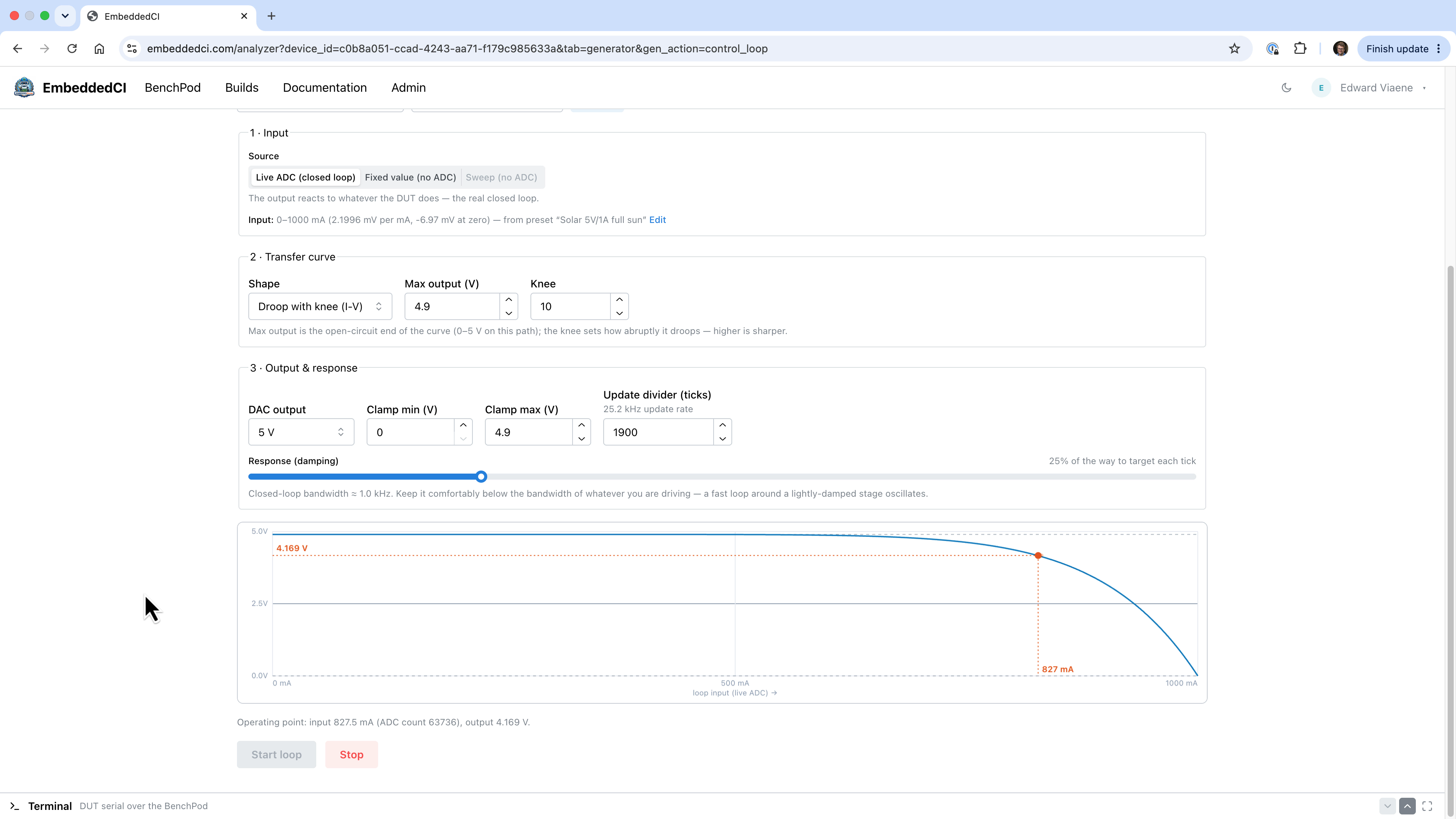
It settles at 827 mA @ 4.169 V, a sag of about 730 mV from open circuit. The load is only drawing 83% of the panel's short-circuit current, so the curve is still fairly flat there and the panel gives away very little voltage. That point also lands at roughly 98% of this panel's maximum power point, so the load happens to be nearly matched.
Half sun
Now the same panel with half the light. Isc halves to 500 mA and Voc drops slightly, which is what really happens: irradiance scales the current almost proportionally, while the open-circuit voltage only falls logarithmically. Modelling shade by lowering Voc is the intuitive move, and it's the wrong one.
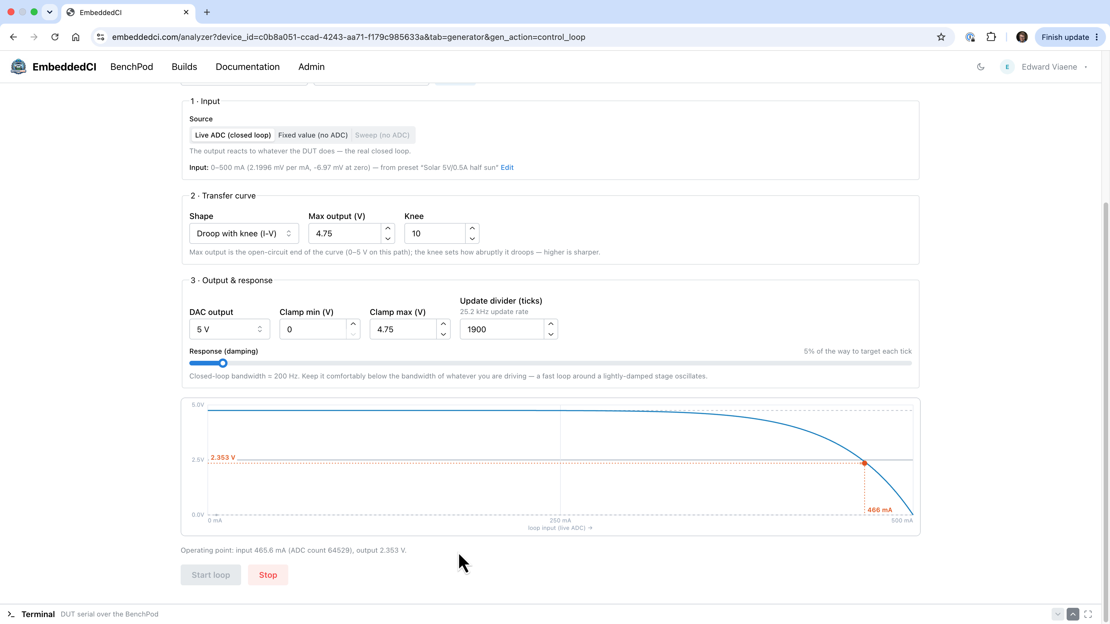
Nothing on the bench moved. The same 5 Ω resistor is still bolted across the same stage. But it now settles at 466 mA @ 2.353 V, a 2.4 V sag, half the panel's open-circuit voltage.
The identical load is now demanding 93% of the panel's remaining short-circuit current, which puts it well over the knee. Ten more points of current draw (83% to 93% of Isc) costs the panel thirty-five points of voltage (15% sag to 50%). That lopsided trade is the knee, and reproducing it is the whole point of the exercise.
It is also a regime change, not just a bigger number. Under full sun the load is voltage-limited: the resistor sets the current at V/R and Isc barely matters. Under half sun it is current-limited: the panel is in charge, and everything downstream has to live with what it can supply. Finding and tracking that transition is exactly what an MPPT algorithm exists to do.
Proving it's the loop, not a weak supply
There is an obvious objection to all this, and it deserves a straight answer. An analog stage that simply can't source enough current also sags under load, and on a plot it looks the same. So how do you know you are seeing an emulated panel rather than an op-amp running out of drive?
Tell the loop to hold a flat curve, the same voltage no matter the current, and measure again. It delivers 966 mA @ 4.86 V, sagging 20 mV. Then switch to the panel curve at the same open-circuit voltage: 826 mA @ 4.15 V, sagging 728 mV.
Same resistor, same rail, seconds apart. The stage had just shown it could supply more current at a higher voltage. Under the panel curve it didn't. The sag is a decision, not a limit.
The loop can go unstable, and the maths tells you when
One more thing worth passing on. The half-sun setup oscillated at first, with the output limit-cycling between 1.92 V and 2.55 V instead of settling.
It isn't mysterious. Linearise the update against a resistive load and the per-tick multiplier is 1 + k(T′ − 1), where T′ is the curve's local slope divided by the load resistance. Under full sun the operating point sits at 83% of Isc where the curve is shallow, giving a multiplier of about 0.31, comfortably stable. Under half sun it sits at 93%, deep on the cliff, where the slope is around six times steeper. The multiplier goes to −1.8, and anything above 1 in magnitude diverges.
The fix is damping, not a different panel. Dropping k from 25% to 5% brought it back to a 20 mV noise floor and the predicted operating point. A steeper curve tolerates less loop gain, which is a useful thing for the emulator to teach you, since a real panel near its knee presents the same problem to whatever is trying to track it.
Why this belongs in CI
A panel simulator turns a category of "we'll find out in the field" behaviour into something a build server can check on every commit:
- Does the charger find the maximum power point, and how close does it get?
- What happens when irradiance halves mid-charge? Does it back off cleanly, or oscillate?
- Does it survive a panel that can't meet its demand, or does it brown out?
- Does firmware that passed last month still behave when the curve moves?
All of it repeatable, and driven from the same API as the rest of the BenchPod. No weather required.
The next step is to swap the resistor for a real solar charger and let two control loops negotiate. A resistor accepts whatever operating point it lands on. An MPPT charger picks one, and watching it hunt across a curve we invented is where this stops being an instrument demo and starts being a test.